Taylor Approximation and JAX

1. Taylor Approximation Review

Taylor’s series allows us to approximate a function 𝑓 as a polynomial, computed using derivatives. In the extrema, if we used infinite coefficients, or up to times that 𝑓 can differentiate, we ended up with a perfect approximation.

\[T_n(x):=\sum_{k=0}^{n}\frac{f^{(k)}(x_0)}{k!}(x-x_0)^k\]

\[T_1(x):= f(x_0) + f^{(1)}(x_0)(x-x_0)\]

Note: 𝑓(𝑘) is 𝑓 differentiate k times, and 𝑘=0 is 𝑓 itself.

Let’s code an example; I will replicate figure 5.4 from the Mathematics for Machine Learning book.

We want to approximate the following function around \(x=0\):

\[f(x) = sin(x) + cos(x)\]

def fun(x): 
    return np.sin(x) + np.cos(x)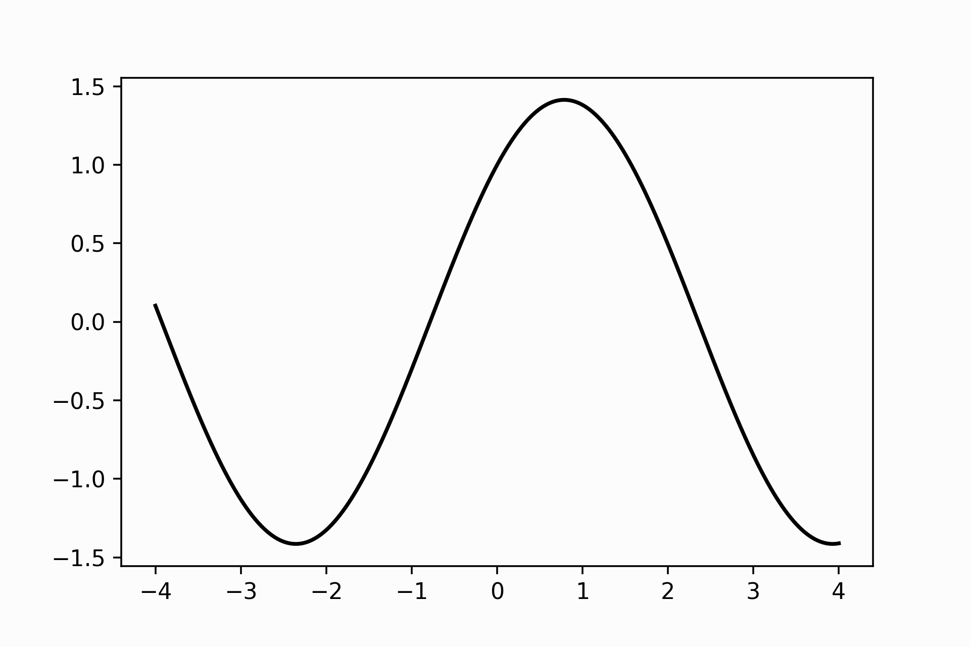

That is like \(f\) looks like around \(x=0\) The task is to get an expression that describes how \(f\) varies around the \(x=0\) neighbourhood. The most straightforward way to achieve this is to remember that \(f'(x)\) is another function that gives us the tangent line at point \(x\). We finish our task; we get an approximation of \(f\) just giving the equation of the tangent line at 𝑥. Knowing what’s the derivative of \(sin\) and \(cos\) plus the addition rule for differentiating, we can compute this manually:

\[f'(x)=cos(x)-sin(x)\]

# Evaluating f`at x=0
np.cos(0) - np.sin(0)
> 1.0

And we get the equation for the tangent line approximating at \(x_0=0\), \(y=f(0)=1\), and \(m=f'(x_0=0)=1\):

\[y - y_0 = m (x - x_0)\]
\[y = 1 + f'(x_0)x\]
\[y = 1 + x\]

taylor_approx(fun, approx_around = 0.0, num_coef=2)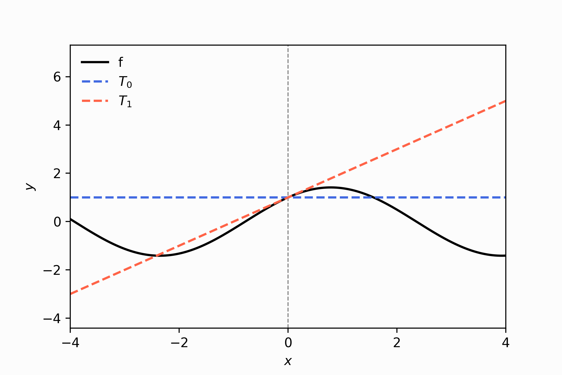

Notice that the tangent line is a pretty good approximation in the immediate space around \(x=0\), but we want something that goes beyond our block. Our approximation gets higher errors when we cross the street at the corner (look at \(x=2\)!).

If we want to be famous at a scale, we need to improve our approximation. To do that, we can improve how we deal with the curvature.

taylor_approx(fun, approx_around = 0.0, num_coef=3, PLOT_COEF = (0,1,2))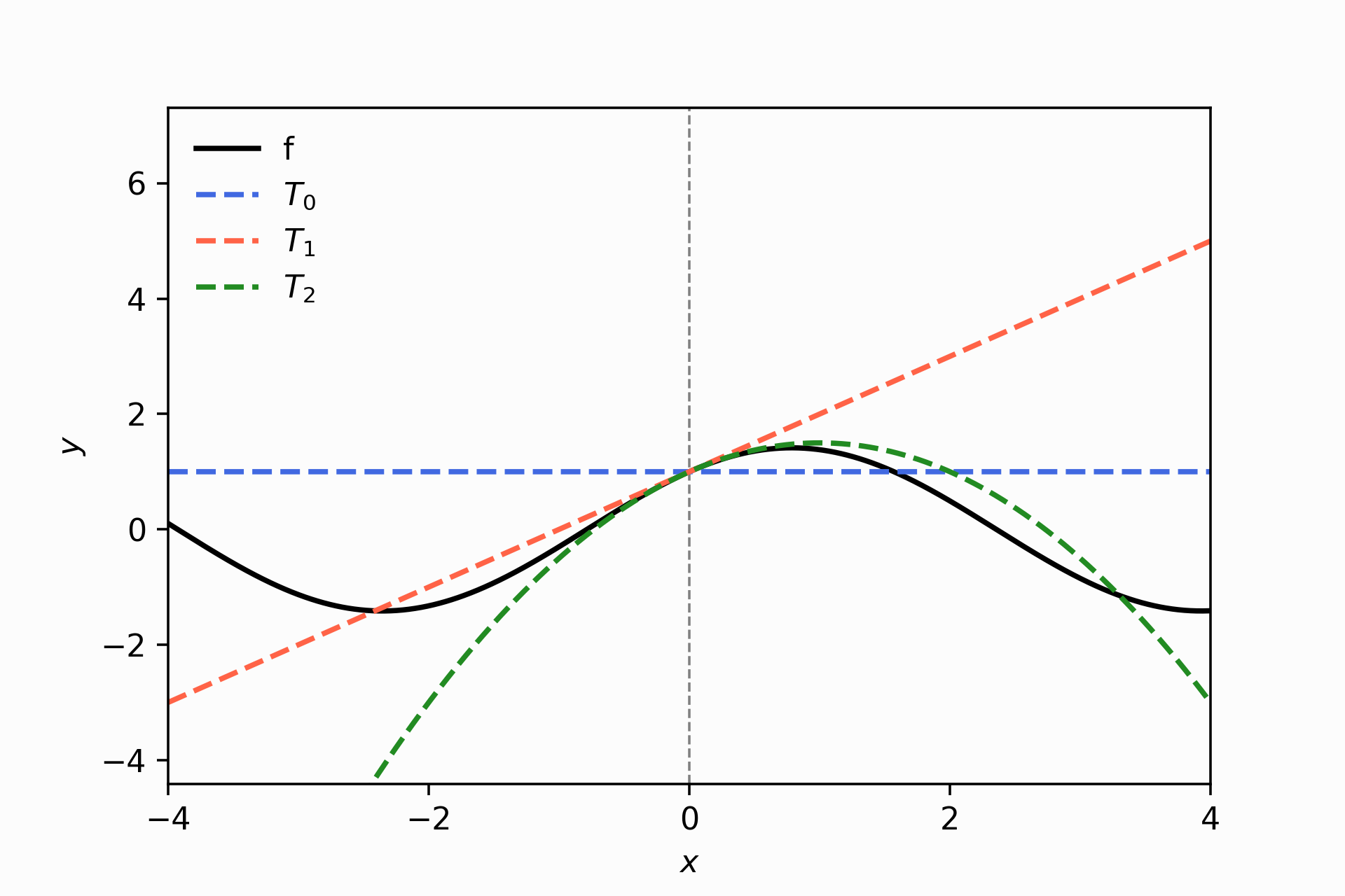

The green line does a better job approximating \(f\) within -1 and 1 than the line. It was intuitive to get an expression for the tangent line, not a quadratic one. How do we get the equation that describes the green line?

Here is when Taylor’s polynomial series is pretty handy:

\[T_2(x):=\sum_{k=0}^{2}\frac{f^{(k)}(x_0)}{k!}(x-x_0)^k\]

To our line equation, we need to add the last term describes in \(T_2\). To obtain this term, we need to compute \(f''\).

In this case, the second derivative is easily computable given that the derivatives are also cyclical because of the nature of \(sin\) and \(cos\):

\(f''=\frac{\partial^2f}{\partial x^2}=\frac{\partial^2}{\partial x^2}\big(sin(x) + cos(x)\big)\)

\(f''=-sin(x)-cos(x)\)

The quadratic approximation or the second-order Taylor approximation is:

\[T_2(x) = 1 + x + \frac{f''(x_0)}{2}x^2\]

# Evaluating f'' at x=0
-np.sin(0) - np.cos(0)
> -1.0

\[T_2(x) = 1 + x -\frac{1}{2}x^2\] It makes sense with the above pictures because the coefficient accompanied by the quadratic term is negative, and therefore we have a concave down curve. Like you can see.

plt.plot(x_jnp, 1 + x_jnp - 0.5 * x_jnp ** 2, 
         color='forestgreen',
         linestyle='-')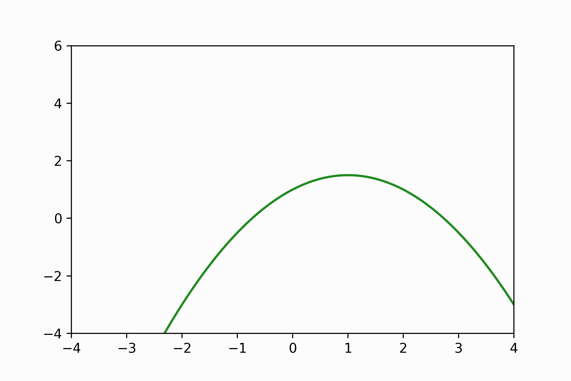

So we can continue repeating this process, adding more coefficients and getting a more accurate approximation. Of course, at the cost of computing higher-order derivatives.

The below image is the final reproduction of figure 5.4. Notice the power of 10 Taylor coefficients (red curve); it approximate \(f\) within the domain interval -4 and 4 almost perfectly. Be cautious, the same that happens with the fifth-order Taylor approximation (green curve), which distances from \(f\) in both lateral of the plot; it would happen to \(T_{10}\) if we expand the x-domain region in the plot.

taylor_approx(fun, approx_around = 0.0, num_coef=11)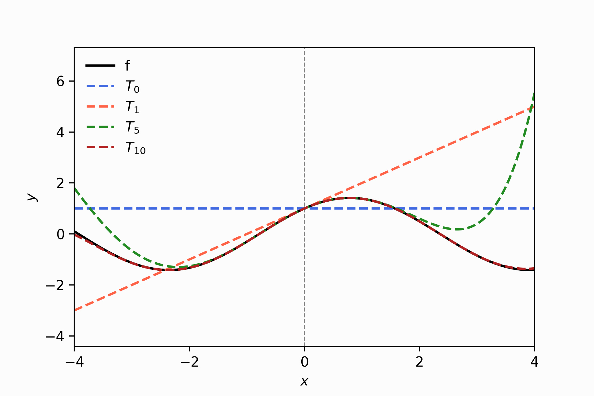

Some thoughts about this section.

1. How can we differentiate any 𝑓 no matter its complexity without relying on manual computations?

2. How can we express the differentiation operations in code?

3. How can we extend Taylor approximation to multivariate functions (i.e. \(f(x_1, \dots, x_n)\)) and everything which involve gradients?

2. Introducing Automatic Differentiation with JAX

JAX is a python library that combines the numpy’s interface, automatic differentiation capabilities, and high-performance operations using XLA and GPU operations.

In this section, we will focus on the fundamentals of JAX to illustrate how to perform automatic differentiation and understand how JAX operates at a high level.

1. jax.grad(): given a function \(f(x)\) implemented in code, it returns a function for compute the gradient (\(f'(x)\))
2. jax.vmap(): vectorize a jax.grad’s function
3. jax.jit(): accelerate a function computations using XLA

Let’s start with an example used by the autograd library, the predecessor of JAX: differentiate the hyperbolic tangent function.

The example is very illustrative because it is apparent how jax.grad works modifying functions; look at the code!

from jax import grad, vmap, jit

@jax.jit
def tanh(x):
    return (1.0 - jnp.exp(-x))  / (1.0 + jnp.exp(-x))

x = jnp.linspace(-7, 7, 200)
fig, ax = plt.subplots(1, 2, sharey=True, figsize=(12.5, 4.5))
ax[0].plot(x, tanh(x), linestyle='-', color='black')
ax[0].axis('off')
ax[1].plot(x, tanh(x),
           x, vmap(grad(tanh))(x),                               # 1st derivative
           x, vmap(grad(grad(tanh)))(x),                         # 2nd derivative
           x, vmap(grad(grad(grad(tanh))))(x),                   # 3rd derivative
           x, vmap(grad(grad(grad(grad(tanh)))))(x),             # 4th derivative
           x, vmap(grad(grad(grad(grad(grad(tanh))))))(x),       # 5th derivative
           x, vmap(grad(grad(grad(grad(grad(grad(tanh)))))))(x)) # 6th derivative
plt.suptitle('tanh and its higher-order derivatives (up to 6th)')           
fig.text(0.75, .02, "Source: Autograd README", size=9, style='italic')
ax[1].axis('off')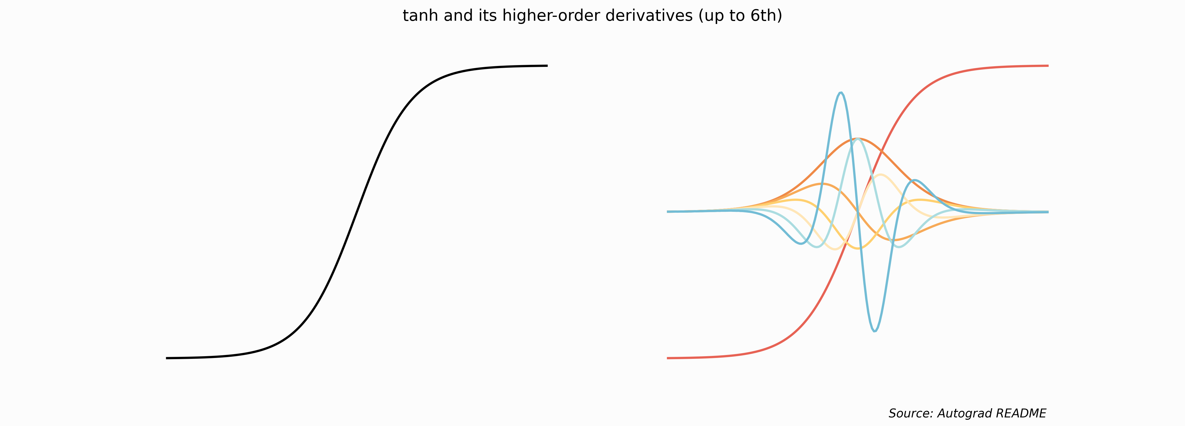

As you can see in the code, grad(tanh) gives you a function to compute the first derivative of tanh. Therefore, the transformation of jax.grad in math notation is the following.

\[(\nabla f)(x)_i = \frac{\partial f}{\partial x_i}(x)\]

Another interesting point is that jax.grad allows you to compose functions in a series of transformations, such as the nested grad application to compute the higher-order derivatives of tanh.

Why is the purpose of jax.vmap? If we want that the function that jax.grad returns behave like this:

tanh(jnp.array([1.0, 2.0,3.0]))
> DeviceArray([0.46211717, 0.7615941 , 0.90514827], dtype=float32)

We need to vectorize the function. Otherwise, we will have an error.

grad(tanh)(1.0)
#grad(tanh)(jnp.arange(10)) # throw an error
> DeviceArray(0.39322388, dtype=float32)

Therefore, if we want to evaluate the gradient at multiple values and receive an array with the results, we can use jax.vmap to transform the function into a vectorize version as much as grad operates modifying functions.

vmap(grad(tanh))(jnp.array([1.0, 2.0, 3.0]))
> DeviceArray([0.39322388, 0.20998716, 0.09035333], dtype=float32)

We can code a naive implementation of jax.vmap to understand what happens behind the scene. Beware that the original function is far more complex, but this is fair to illustrate the main functionality.

def my_vmap(x, grad):
  """A basic implementation of vmap to vectorize a function""" 
  FUN = grad
  out = []
  for i in range(x.shape[0]):
    out.append(FUN(x[i]))
  return jnp.array(out)
  
my_vmap(jnp.array([1.0, 2.0, 3.0]), grad(tanh))
> DeviceArray([0.39322388, 0.20998716, 0.09035333], dtype=float32)

You have an idea of how I replicate figure 5.4 of the previous sections that require computing up to a tenth-order Taylor approximation. Yes, it’s unnecessary to hand-code the derivatives. I just used jax.grad ten times over \(f\) itself.

NABLA = FUN
for i in range(NUM):
  # Compute the ith derivative of FUN
  NABLA = jax.grad(NABLA)
  # Do something like computing the ith taylor coefficient
  ...

For instance, let’s plot tanh and its derivatives, but this time we will differentiate ten times using the above pattern and avoid the nested code’s boilerplate.

NABLA = tanh
for i in range(10):
  plt.plot(x, vmap(NABLA)(x))
  NABLA = grad(NABLA)
plt.axis('off')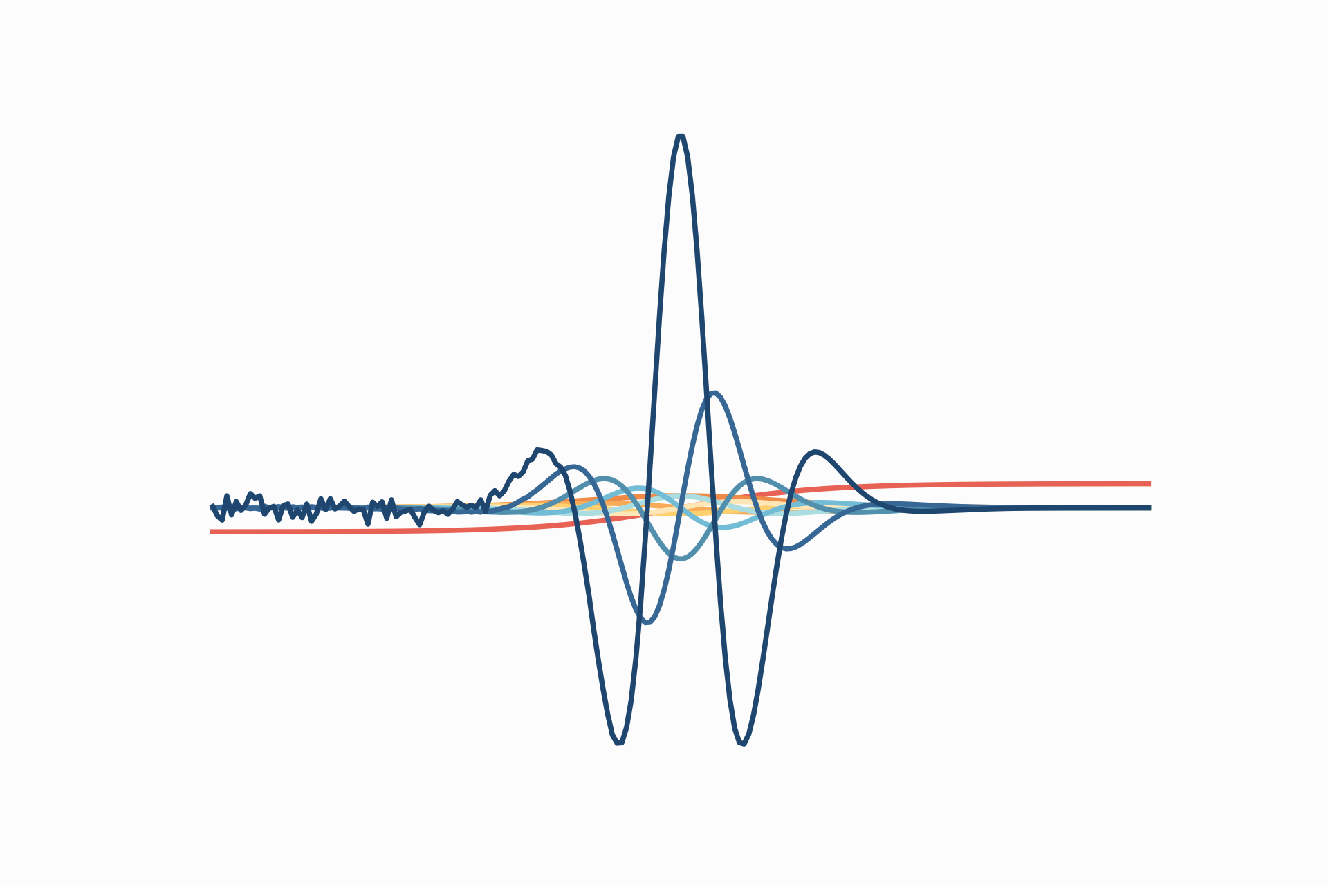

Computing higher-order derivatives can be computationally expensive. Read the paper “Taylor-Mode Automatic Differentiation for Higher-Order Derivatives in JAX” to understand the efficient way to compute higher-order derivatives. More context about this problem and the paper’s genesis in this discussion.

How are the derivatives computed? JAX allow us to perform automatic differentiation and calculates results transforming numerical functions into a directed acyclic graph (DAG):

• outer lefts nodes represent the input variables
• middle nodes represent intermediate variables
• the outer right nodes represents the output node (a scalar)
• as the name said, there are no cycles in the graph; the data always flows from left to the right, it could have branches, but none edge can point back

The differentiation is just an application of the chain rule over DAG.

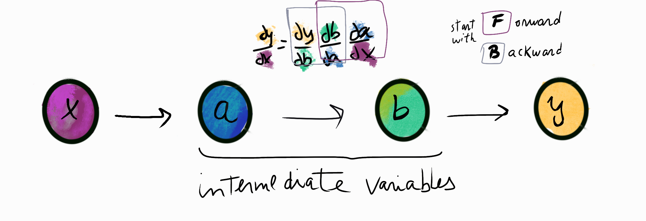
Once we have all the derivatives, we start multiplying but wait, the order matters. Suppose we begin multiplying the square “F”, as the diagram above shows you. Using different orders to compute the gradient can get efficient depending on the problem.

jax.make_jaxpr produces the JAX representation of the computation made, and it helps us visualise the diagram described above.

The intermediate variables are equations (jaxpr.eqns) that receive inputs, could be the function’s input or other intermediate variables, and a set of primitive operations to compute over these to produce outputs.

You can read more about jax.make_jaxpr in the documentation.

For instance, we can inspect how JAX decouples the function \(f(x)=x^2 + exp(x)\) in intermediate variables.

def f(x):
  return x**2 + jnp.exp(x)

jax_compu = jax.make_jaxpr(f)(3.0)
jax_compu
> 
 { lambda ; a:f32[]. let
    b:f32[] = integer_pow[y=2] a
    c:f32[] = exp a
    d:f32[] = add b c
  in (d,) }

We can code a function to extract each element of the above jaxpr.

def describe_jaxpr(FUN):
  """Given a function, print each element of its jaxpr"""
  from inspect import getsource
  print('Source function definition:')
  print(getsource(FUN))
  print('--------------------------------------------------------------')
  # Evaluate the expression on 0.0 (arbitrary) to get a jaxpr
  expr = jax.make_jaxpr(FUN)(0.0).jaxpr
  print('The function has the following inputs, represented as ' + str(expr.invars))
  print('the function has the following constants, represented as ' + str(expr.constvars))
  # Get the equation that describe each intermediate variable and extract info 
  print('\nThese are the intermediate variables describe by the equations computed along the DAG: ')
  for i, eq in enumerate(expr.eqns):
    print('   ' + str(i) + '. ' + 'Obtain ' + str(eq[1]) + ' applying the primitive ' + str(eq.primitive) + ' with params ' + str(eq.params) + ' on input/s ' + str(eq[0]))
  print('\n The output is: ' + str(expr.outvars)) 

describe_jaxpr(f)
> 
Source function definition:
def f(x):
 return x**2 + jnp.exp(x)

--------------------------------------------------------------
The function has the following inputs, represented as [a]
the function has the following constants, represented as []

These are the intermediate variables describe by the equations computed along the DAG: 
  0. Obtain [b] applying the primitive integer_pow with params {'y': 2} on input/s [a]
  1. Obtain [c] applying the primitive exp with params {} on input/s [a]
  2. Obtain [d] applying the primitive add with params {} on input/s [b, c]

The output is: [d]

Similar to the diagram above, we have two intermediate variables used to describe the output in this example.

• Input \(x\) is represented by \(a\)
• The first intermediate variable is \(b=a^2\)
• Then, the second intermediate variable is created also using as input \(a\): \(c=exp(a)\)
• Finally, the output is computed by summing the two intermediate variables: \(d=b+c\).

Similarly, we can inspect the gradient function of \(f\) given by jax.grad(f):

describe_jaxpr(jax.grad(f))
> 
Source function definition:
def f(x):
  return x**2 + jnp.exp(x)

--------------------------------------------------------------
The function has the following inputs, represented as [a]
the function has the following constants, represented as []

These are the intermediate variables describe by the equations computed along the DAG: 
   0. Obtain [b] applying the primitive integer_pow with params {'y': 2} on input/s [a]
   1. Obtain [c] applying the primitive integer_pow with params {'y': 1} on input/s [a]
   2. Obtain [d] applying the primitive mul with params {} on input/s [2.0, c]
   3. Obtain [e] applying the primitive exp with params {} on input/s [a]
   4. Obtain [_] applying the primitive add with params {} on input/s [b, e]
   5. Obtain [f] applying the primitive mul with params {} on input/s [1.0, e]
   6. Obtain [g] applying the primitive mul with params {} on input/s [1.0, d]
   7. Obtain [h] applying the primitive add_any with params {} on input/s [f, g]

 The output is: [h]

Notice that the number of intermediate variables increases. For instance, you can look at the equation described in (2) that is a primitive adding resulting from the differentiation: \(\partial/\partial x (x^2)\rightarrow 2x\).

Further resources on automatic differentiation and JAX:

1. What’s automatic differentiation video
2. JAX’s tutorial by Mat Kelcey showing more about parallel computing using JAX
3. Automatic Differentiation, Deep Learning Summer School Montreal 2017 (Matthew Jonhson); another seminar about the topic JAX seminar

3. Taylor Approximation with two variables

Now we consider the setting when functions are multivariate:

\[f: ℝ^D ⟶ ℝ\] \[\quad \quad \quad \quad \quad \quad x ↦ f(x), \quad x \in ℝ^D\]

By definition 5.8 in MML, we have that a Taylor approximation of degree n is defined as:

\[T_n(x)=\sum^{n}_{k=0}\frac{D^k_x f(x_0)}{k!} 𝜹^k\]

The vector \(𝜹\) represents a difference between \(x\) and \(x_0\); the latter is a pivot-vector in which the approximation is around made.

\(D^k_x\) and \(𝝳^k\) are tensors or k-dimensionl arrays.

November 10, 2020

If we have that \(𝛅 \in ℝ^4\), we obtain \(𝛅^2:=𝛅⨂𝛅=𝛅𝛅^T ∈ ℝ^{4x4}\)

delta=jnp.aarange(4)   # this is [0, 1, 2, 3]
jnp.eisum('i,j', delta, delta)
DeviceArray([[0, 0, 0, 0],
             [0, 1, 2, 3],
             [0, 2, 4, 6],
             [0, 3, 6, 9]], dtype=int32)

\(𝛅^3:=𝛅⨂𝛅⨂𝛅\in ℝ^{4x4x4}\)

jnp.eisum('i,j,k', delta, delta, delta)
DeviceArray([[[ 0,  0,  0,  0],
              [ 0,  0,  0,  0],
              [ 0,  0,  0,  0],
              [ 0,  0,  0,  0]],

             [[ 0,  0,  0,  0],
              [ 0,  1,  2,  3],
              [ 0,  2,  4,  6],
              [ 0,  3,  6,  9]],

             [[ 0,  0,  0,  0],
              [ 0,  2,  4,  6],
              [ 0,  4,  8, 12],
              [ 0,  6, 12, 18]],

             [[ 0,  0,  0,  0],
              [ 0,  3,  6,  9],
              [ 0,  6, 12, 18],
              [ 0,  9, 18, 27]]], dtype=int32)

For instance, in the last 4x4x4 array, the last number computed is 64 by delta[3]*delta[3]*delta[3] (4x4x4). Instead, the most lower-left element of the third 4x4 array is 48 and you obtained it by delta[2]*delta[3]*delta[3] (3x4x4).

The Einstein Summation implemented in jnp.einsum is a notation that allow you to represent a lot of array operations using index notation. Look this video for a detail explanation and the documentation.

Let’s code the example 5.15, deriving at first manually and then use JAX to check if we reach similar results.

def g(x, y): 
    """Function used in the example 5.15 in MML"""  
    return x ** 2 + 2 * x * y + y **3

x = jnp.linspace(-5, 5, 50)
y = jnp.linspace(-5, 5, 40)
X, Y = np.meshgrid(x, y)
Z = g(X, Y)

fig = plt.figure(figsize = (7.2, 4.3))
ax = fig.add_subplot(1, 1, 1, projection='3d')
ax.set_title("$g(x,y)=x^2+2xy+y^3$")
ax.plot_surface(X, Y, Z, rstride = 3, cstride = 3, cmap = 'cividis',
                antialiased=False, alpha=.6)
ax.set_xlabel('x')
ax.set_ylabel('y')
ax.set_zlabel('z')
ax.zaxis.set_major_locator(
plt.MultipleLocator(60))
plt.subplots_adjust(left=0.0)
ax.view_init(15, 45)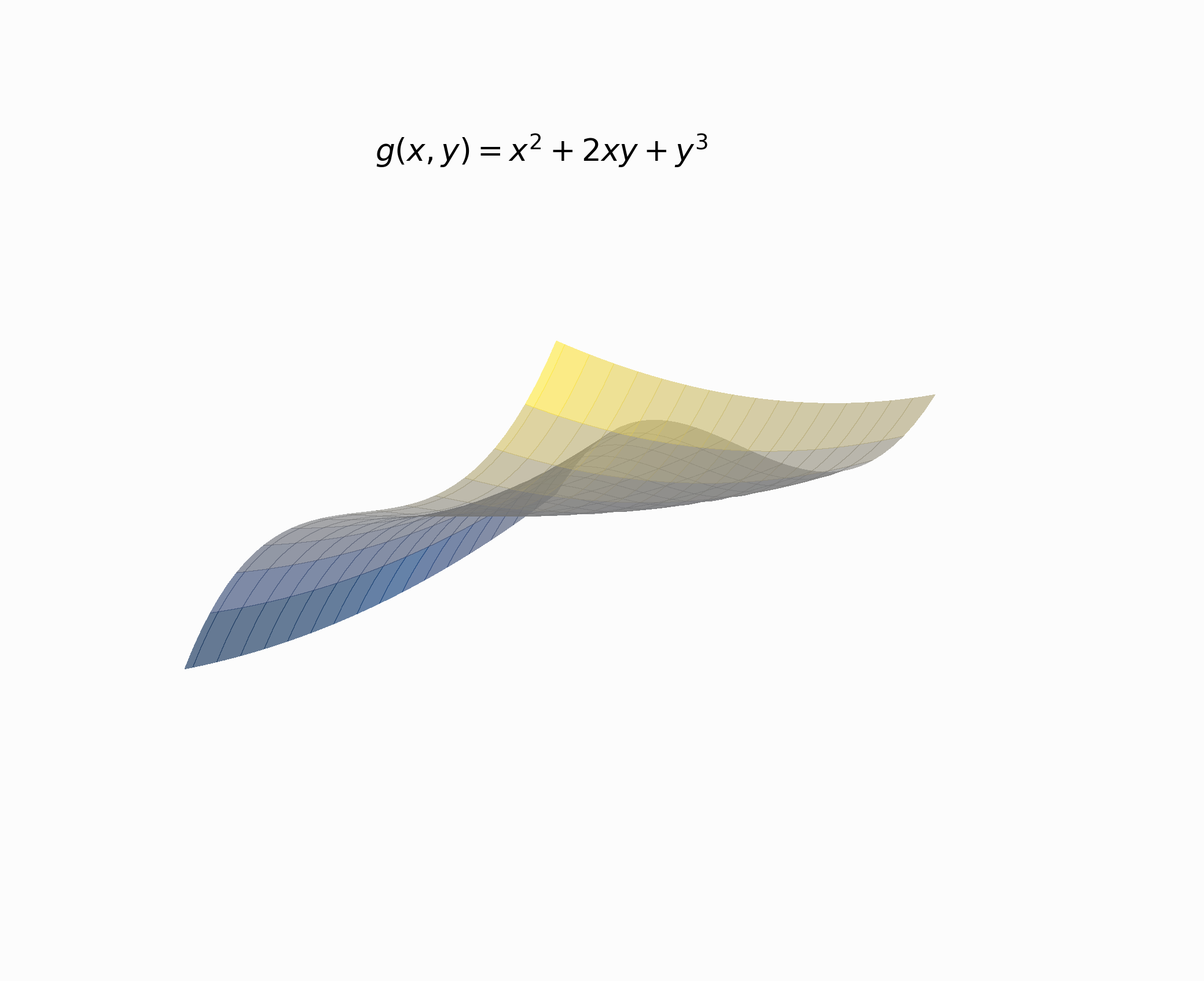

We will start with the first-order Taylor approximation, which gives us a plane.

We need \(\partial g/ \partial x\) and \(\partial g/ \partial y\) collect the gradient into a vector (aka jacobian vector) and multiply by \(𝛅\).

\[\partial g/\partial x=2x+2y\] \[\partial g/ \partial y=2x+3y^2\]

Collect the partials into a vector:

\[D^1_x=\nabla_{x,y}=\big[2x+2y \quad 2x+3y^2\big]\]

Following the instruction of the example, we will approximate around \((x_0, y_0)=(1,2)\).

Now we can evaluate all the expressions for completing the equation that describes the plane:

\[T_1(x, y)=f(x_0, y_0) + \frac{D^1_x f(x_0, y_0)}{1!} 𝜹^1\]

def dg_dx(x,y): 
  """Derivative of g() w.r.t x hand-coded"""
  return 2*x + 2*y
  
def dg_dy(x,y): 
  """Derivative of g() w.r.t y hand-coded"""
  return 2*x + 3*y**2

print('g(1,2): ' + str(g(1,2)))
print('dg/dx(1,2): ' + str(dg_dx(1,2)))
print('dg/dx(1,2): ' + str(dg_dy(1,2)))
> g(1,2): 13
> dg/dx(1,2): 6
> dg/dx(1,2): 14

\[T_1(x, y)=13 + [6 \quad 14] \begin{bmatrix} x-1 \cr y-2 \end{bmatrix}\]

\[T_1(x, y)=13 + 6(x-1) + 14(y-2)\]

\[T_1(x, y)=6x+14y-21\]

def g_plane_approx(x, y):
    """Equation that describe the tangent plane at g(1,2)"""
    return 6*x + 14*y - 21 

Similar to the 1D case, but now the line is a plane. You can notice that is a good approximation at the very close neighbourhood of the point \((x_0, y_0)=(1,2)\). However, the plane fails to approximate the curvatures of \(g\).

Now with autodiff…how can we compute the jacobian vector? We can save all the hand-coded derivatives using the function jax.grad.

jax.asarray(jax.grad(g, argnums=(0,1))(1.0, 2.0))
> DeviceArray([ 6., 14.], dtype=float32

There is another way to get the jacobian.

jnp.asarray(jax.jacfwd(g, argnums=(0,1))(1.0, 2.0))

jax.jacfwd’s name stands for jacobian forward and refers to the order that computes the chain rule. We can use jax.jacrev to obtain the same results but traverse the graph backwards. There is no concern about which one to use in this example because the function g is straightforward in complexity. Still, it matters when many variables are involved, and as a result, we get different shapes of the jacobian matrix.

jnp.asarray(jax.jacrev(g, argnums=(0,1))(1., 2.))

The argument argnums specified which with argument differentiate the function. We give a tuple with the only two arguments of g(x,y), i.e. I want the full jacobian vector that has the gradient w.r.t. argument 0 (x) and argument 1 (y).

For example, lets compute the jacobian vector for \(x^2+3y+z^2\) and evaluate the gradient \((1.0, 2.0, 2.0)\).

jnp.asarray(
            jax.jacfwd(lambda x, y, z: x**2 + 3*y + z**2, 
                                         argnums=(0,1,2))(1.0, 2.0, 2.0)
            )
> DeviceArray([2., 3., 4.], dtype=float32)

Note: jax.asarray collect all the derivatives in a single flat array.

How can we go further computing the Hessian?

We compute the second-order derivatives of \(g\) and collect them into the \(H\) matrix.

\[H= \left(\begin{matrix} \frac{\partial^2 g}{\partial x^2}=2 & \frac{\partial^2 g}{\partial xy}=2 \\ \frac{\partial^2 g}{\partial yx}=2 & \frac{\partial^2 g}{\partial y^2}=6y \end{matrix} \right)\]

There are three constants except for the lower-right element of \(H\). We can compute \(H\) with two passes of jacfwd and evaluate (1,2) to obtain the Hessian matrix.

H = jnp.asarray(jax.jacfwd(jax.jacfwd(g, argnums=(0,1)), argnums=(0,1))(1., 2.))
H
> DeviceArray([[ 2.,  2.],
               [ 2., 12.]], dtype=float32)

There is multiple ways to compute the second Taylor’s polynomial coefficient using the Hessian.

delta = jnp.array([1., 1.]) -  jnp.array([1.0, 2.0])
jnp.trace(0.5 * [email protected]('i,j', delta, delta))
> DeviceArray(6., dtype=float32)

0.5 * jnp.einsum('ij,i,j', H, delta, delta)
> DeviceArray(6., dtype=float32)

Ok, now we will code a function to compute the Taylor approximation using the above knowledge.

def quadratic_taylor_approx(FUN, approx, around_to):
  """Compute the quadratic taylor approximation for the set of points 'approx' of a given FUN around the. point 'around_to'"""
  delta = approx - around_to
  # Compute the Jacobian and the linear component
  J = jnp.asarray(jax.jacfwd(FUN, argnums=(0,1))(*around_to))
  linear_component = J.dot(delta.T)
  # Compute the Hessian and the qudractic component
  H = jnp.asarray(
                  jax.jacfwd(
                            jax.jacfwd(FUN, argnums=(0,1)), 
                            argnums=(0,1)
                            )(*around_to)
                  )
  quadratic_component = 0.5 * jnp.einsum('ij, ij->i', 
                                         jnp.einsum('ij,jk->ik', delta,H), 
                                         delta)
  return FUN(*around_to) + linear_component + quadratic_component

quadratic_taylor_approx(g, jnp.array([[1.0, 1.0], [1.0, 2.0], [3.0, 4.0]]), jnp.array([1.0, 2.0]))
> DeviceArray([ 5., 13., 89.], dtype=float32)

The quadratic component (aka second order derivatives) gives us a better way to approximate the curvature of \(g\).

Visually it looks ok, but we can use the closed-form expression for the quadratic Taylor approximation around the point \((1, 2)\) to verify if the function quadratic_taylor_approx is doing its job.

Note: You can work out the closed-form expression from equation 5.180c in MML, and ignore the third-order partial derivatives.

\[T_2(x, y)=x^2+6y^2-12y+2xy+8\]

def g_quadratic_approx(x, y):
  """Close-form expression for the quadratic taylor approx of g() around (1, 2)"""
  return x**2 + 6*y**2 - 12*y + 2*x*y + 8

# Some cases to test
print(g_quadratic_approx(1.0, 2.0))
print(g_quadratic_approx(2.0, 3.0))
print(g_quadratic_approx(4.2, 3.7))
print(g_quadratic_approx(2.8, 1.3))
print(g_quadratic_approx(10.2, 21))
print(g_quadratic_approx(-5.1, 2.3))
print(g_quadratic_approx(-3.4, -2.5))
> 13.0
> 42.0
> 94.46000000000001
> 17.659999999999997
> 2934.44
> 14.689999999999998
> 104.06

quadratic_taylor_approx(g, jnp.array([[1.0, 2.0], 
                                      [2.0, 3.0],
                                      [4.2, 3.7],
                                      [2.8, 1.3],
                                      [10.2, 21],
                                      [-5.1, 2.3],
                                      [-3.4, -2.5]
                                      ]), 
                        around_to=jnp.array([1.0, 2.0]))
> DeviceArray([  13.      ,   42.      ,   94.46    ,   17.659998,
             2934.44    ,   14.690002,  104.05999 ], dtype=float32)

The values are practically the same. There are some cases with approximation error around the thousandth.