Ukiyo-e style postcard generator App

What is Ukiyo-e style?

Pictures-of-the-floating-world…, that’s what means the Japanese word Ukiyo-e. It’s a term to refer to an entire art gender, so don’t be confused that it is an artist’s name or a pseudonym. Its roots are popular, even vulgar, and accessible, so it was easy to find Ukiyo-e prints in Japanese houses. It was a genre that took influence from the west and china, but at some point, it influenced Europe and the western world. If you want to know more about this Japanese art genre, I highly recommend this interactive piece from the New York Times titled A Picture of Change for a World in Constant Motion" (Farago 2020). It’s a journey from this popular genre’s history and distinctive elements.

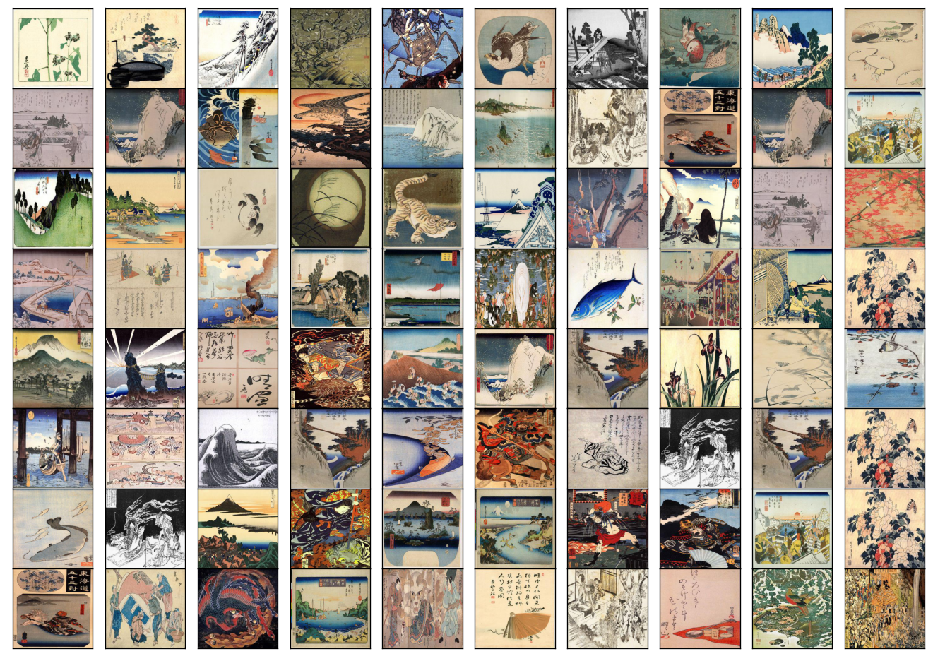
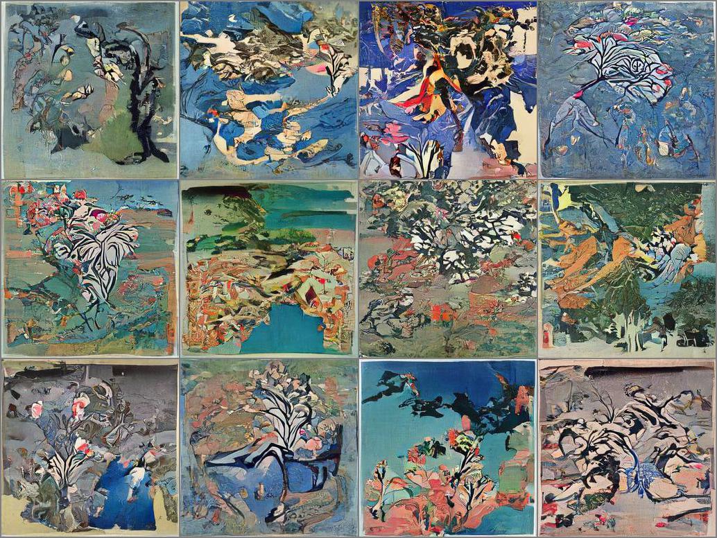
The dataset ukiyoe2photo contains pictures of the floating world, which I used in this project to learn a model to generate new images with ukiyo-e stylish. The below figure shows some of the ukiyo-e images in the dataset.

Unconditional image generation

What is unconditional image generation?

Unconditional image generation is the task of generating images with no condition in any context (like a prompt text or another image). Once trained, the model will create images that resemble its training data distribution.

My goal here is to highlight the main elements involved in a Denoising Diffusion Probabilistic Model (Ho 2020), or DDPM for short, and its training dynamic. I will write a more detailed and technical post about this model in the future.

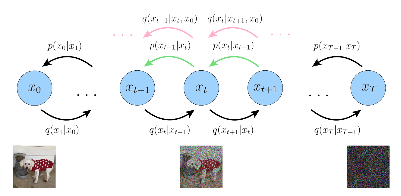
Let’s start with the training dynamic; a diffusion model consists of two chain processes of the same number of steps, \(T\).

1. A forward process: in which the model takes an input image and gradually destroys it, adding gaussian noise until the entire image structure is reduced to just noise
2. And a backward process: an inverse process encoded by a distribution with learnable parameters whose goal is to predict the noise added in each transition step (i.e. denoising)

There are important elements to take into account:

• We use gaussian distributions for both processes, yeah the lovely normal distribution \(\mathcal{N}(\mu, \sigma)\)
• Both processes are markovian; that means the distribution of a given step t depends on the immediately previous state \(t-1\) or \(t+1\) in the case of the backward process
• The gaussian distribution of the forward process (\(q(\cdot)\) in the above diagram) has fixed parameters; in other words, we don’t have to learn any parameter here
• In contrast, the gaussian distribution for the backward process (\(p_{\theta}(\cdot)\) in the diagram) has learnable parameters \(\boldsymbol \theta\)
• We used a noise schedule to destroy the images; this means that we have a deterministic function to inject the amount of noise during the \(T\)-length forward process
• We used a neural network architecture (e.g. U-net) to predict the parameters of the backward gaussian distribution \(p_{\boldsymbol \theta}\)
• If we have a process of length \(T=1000\) (like Ho 2020), \(\boldsymbol x_{0}\) is the image input, \(\boldsymbol x_{1000}\) is pure noise of the same input resolution, and any intermediate \(\boldsymbol x_t\) with \(0\lt t \lt T\) is a latent state; a blend of some degree between the input image and noise level (given by the noise scheduler)
• The last means that every latent space has the same resolutions as the input (a difference from other variational autoencoder models)
• The advantage of using a noise scheduler + gaussian distribution with known parameters \(q(\cdot)\) is that we have a closed expression to compute the latent state at any given level \(t\) (we don’t need to calculate the entire chain from \(0\) to \(t\)).

Back to the training dynamic, a one parameter update cycle looks like the following:

1. Get a batch of images \(\mathrm{x}\) from our dataset (batch_size, width, height)
2. Sample random gaussian noise \(\mathrm{\epsilon}\) for each image (batch_size, width, height)
3. Pick a random vector \(\mathrm{t}\), which determine in which part of the forward process we are for each of the images (batch_tize,) (think we are extending parallel non-equal length chains)
4. Compute the latent state \(\mathrm{z}\): each image in the batch use their corresponding \(t\) level in \(\mathrm{t}\) with the closed expression. The noise scheduler knows how to blend the image with the noise at the right level (batch_size, width, height)
5. Pass \(\mathrm{z}\) for the model \(p_{\boldsymbol \theta}\) to get the predicted noise \(\epsilon^{*}\)
6. Using the mean squared error as a loss function, we compare the actual noise (\(\mathrm{\epsilon}\)) with the predicted noise (\(\mathrm{\epsilon}^{*}\)). Remember that we know the actual noise beforehand because our noise schedule needs it to blend it with the image and create the latent state.
7. Backprop to compute the gradients
8. Update the parameters in the direction that minimizes the loss

num_epochs = 1  # number of epochs
lr = 1e-5  # learning rate
grad_accumulation_steps = 2  # how many batches to accumulate the gradient before the update step
optimizer = torch.optim.AdamW(image_pipe.unet.parameters(), lr=lr)

for epoch in range(num_epochs):
    for step, batch in tqdm(enumerate(train_dataloader), total=len(train_dataloader)):
        # get a batch image 
        clean_images = batch["images"].to(device)
        # Sample noise to add to the images
        noise = torch.randn(clean_images.shape).to(clean_images.device)
        bs = clean_images.shape[0]

        # Sample a random timestep for each image
        timesteps = torch.randint(
            0,
            image_pipe.scheduler.num_train_timesteps,
            (bs,),
            device=clean_images.device,
        ).long()

        # Add noise to the clean images according to the noise magnitude at each timestep
        # (this is the forward diffusion process)
        noisy_images = image_pipe.scheduler.add_noise(clean_images, noise, timesteps)

        # Get the model prediction for the noise
        noise_pred = image_pipe.unet(noisy_images, timesteps, return_dict=False)[0]

        # Compare the prediction with the actual noise:
        loss = F.mse_loss(
            noise_pred, noise
        )  

        # Update the model parameters with the optimizer based on this loss
        loss.backward(loss)

        # Gradient accumulation:
        if (step + 1) % grad_accumulation_steps == 0:
            optimizer.step()
            optimizer.zero_grad()

It looks straightforward, but there are many theoretical building blocks to end using a mean squared error loss. The code above uses the hugging face diffuser library 🧨, so some lines are more complex—for instance, image_pipe.scheduler_add_noise knows exactly how to blend the images with the noise to get a determined latent state at \(t\). It’s initialized before with the \(T\) length, noise schedule type, etc. The object image_pipe.unet contains the neural network architecture to process the images; remember that the latent space is of the same shape that the input (i.e. image). The last explained the decision by the authors to choose a U-net architecture, well known because the output has the exact dimensions as the input.

Training a generative model such as DDPM takes a long time and requires a lot of images. Instead, we can get fair results without much training and pictures using the same approach but with a pre-trained model as a starting point, such as Google/ddpm-celebahq-256. Of course, we need to make some compromises to the model resolutions we are using to finetune our data; the Google model was trained using a 256px resolution.

Now we can use the model to sample 12 postcards:

x = torch.randn(12, 3, 256, 256).to(device)  # Batch of 12 
for i, t in tqdm(enumerate(scheduler.timesteps)):
    model_input = scheduler.scale_model_input(x, t)
    with torch.no_grad():
        noise_pred = image_pipe.unet(model_input, t)["sample"]
    x = scheduler.step(noise_pred, t, x).prev_sample

Notice that we need to denoise the gaussian random noise to get samples from the model throughout the backward process chain. In the next section, we will add some complexity to this inference pipeline beyond the model and the noise scheduler. You can find the model used to generate the images in alkzar90/sd-class-ukiyo-e-256.

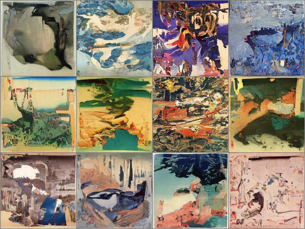
There are psychodelich images, dreamy ones without some realistic object, but still with an artistic appeal. Observe the opaque pastel colours characteristic of the Ukiyo-e style.

Classifier Guidance

What is the guidance technique? We can take this unconditional image generation process and guide it toward images that have a desired attribute or property of interest we want. It could be like conditioning the image distribution hackily because we don’t need to learn the conditional distribution like in popular text-to-image models such as Stable Diffusion or Dall-E2; we reuse the same model. Instead, we guide the sampling process (or denoising) by introducing a loss function that measures the property of interest in the sample generated, orienting the denoising process to minimize the designed objective. Specifically, in the Ukiyo-e style postcard generator App, we used:

• Colour guidance: samples images that have a (guess) desired colour
• Text prompt guidance: sample images according to a text description

So, before we look that generating a new image, or sampling, means taking a pure gaussian noise and passing through this denoising process. But we do it in many little steps; you take the noise and denoising slowly, passing through an entire stochastic Markovian process of saying T=1000 steps (Ho 2020,). When we use guidance, we append a gradient graph to the sample tensor and calculate the loss for the sample in each state w.r.t our objective attribute (e.g. colour or text prompt). Then we compute the gradient and update the tensor in the direction that minimizes the loss, guiding the following sample image to be more appealing to the attribute that measures the loss. The process is called classifier guidance, and it was introduced in the paper Diffusion Models Beat GANs on Image Synthesis (Dhariwal 2021).

Now a beautiful image of a sakura tree…

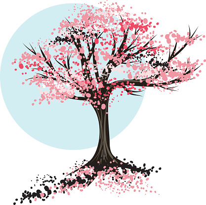
We will use “a sakura tree” as a text prompt and the same starting gaussian noise as above, for which we got 12 ukiyo-e-postcard. But, this time, we will drive the sampling process using the gradients we get by comparing the sample image text encoding in each step \(t\) with the text prompt encoding vector.

Compare these new postcards with the others. Notice how the text guidance makes that sakura tree’s pattern emerge during the denoising process: branches and pink leaves here and there, with hallucination touches. The model is neither perfect nor trained with surgery hands, but it’s still amazing that we have gained some control over the sampling process. Behind the curtains, to generate the above images, the following steps happen:

1. Download a pre-trained model to generate image captions such as OpenAI CLIP model
2. Pass the noise tensor to the model to get an encoding vector
3. Use a loss function that compares the vector for the current sample state w.r.t. encoding for the text prompt; the last vector is always the same because the prompt doesn’t change during the process
4. Compute the sample gradient w.r.t loss value and update the sample values in the direction that minimizes the loss
5. Repeat the process during the whole stochastic Markovian process

Generally, any designed loss uses a scale factor to increase/decrease the attribute effect. It allows you to move between novelty and fidelity. Moreover, there’s nothing to block you from using more than one objective; the Ukiyo-e postcards generator uses colour, and text prompts together as guidance, and each loss contributes to accumulating gradients that modify the sample in each denoising step. Of course, there could be some gradient interaction effects. Imagine that you want green images, but at the same time, you are using the text prompt “a volcano lava” you will put against the red/brown implicit colours in the text prompt with the green one.

Wrap the inference pipeline into an App

Now that we have a trained model and know how to control the sampling process of the unconditional distribution, why not wrap the entire inference pipeline into a friendly interface such as a Gradio App?

Let’s start by setting some context; Gradio is a framework that allows us to build machine-learning apps pretty fast based on the task for which our model was designed. For instance, in a generative image model, in which the inference process requires fixing different parameter types such as factor scale (slider), text prompt (text input), or colour (colour selector), plus we always expect an image as output. Gradio helps us accommodate these requirements, hiding many tedious details that save you valuable time.

In addition, Hugging Face gives you free space to host your App running on a CPU (you can power up the running using a GPU, but you need to pay). It’s an excellent combo to provide you with a friendly web interface with minimal resources. There is a trend in the generative model community for using this interface to show and prototype their models’ properties and features, such as Stable Diffusion 2.1 Demo or Diffuse the rest. Therefore, taking time to learn Gradio is an excellent decision to share your project with a friendly facade.

Here is the python script with the pipeline and the App code, also a screenshoot of how does it look the Ukiyo-e style postcard generator App:

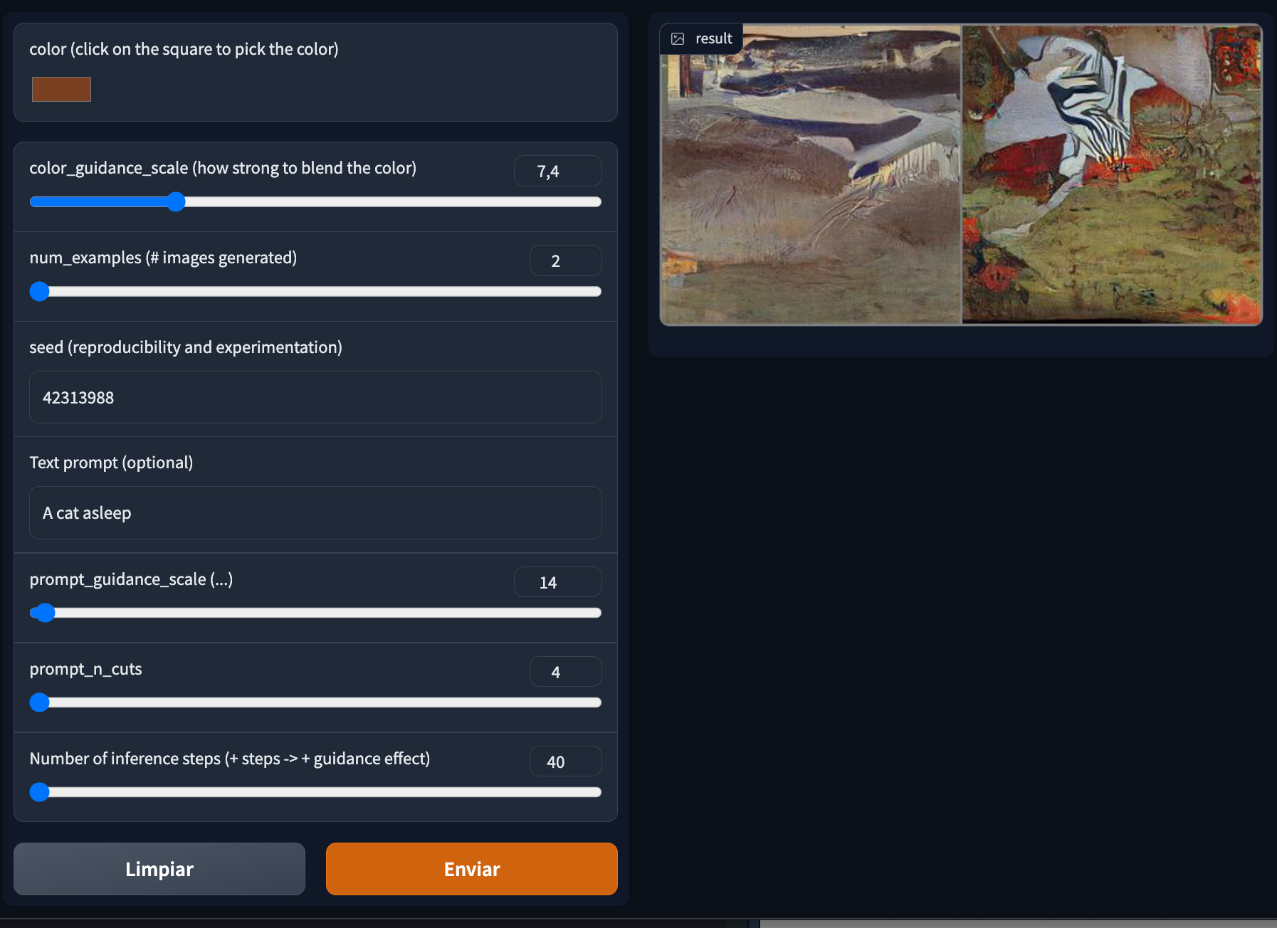
As you can see, it is easier to pick the colour you want and enter a text prompt to guide the sampling; control the scale factors for experimenting with different guidance intensity levels. Using a seed is convenient for reproducing the gaussian noise, which the denoising process use as a starting point for generating the images, so you can edit iteratively the image generated by playing with the scale factors.

PD: Unfortunately, this kind of model involves a lot of computation, and the gradio App is running using huggingface space with CPU, so that means the whole inference pipeline takes a lot of time. But, the good news is if you don’t have patience, you can run the Gradio App using the google colab notebook pointing out at the start of this post with the GPU setting.